Working with databases in R: dplyr

Introduction

In this post I offer an overview of some handy tools for working with databases in R: dplyr/ dbplyr packages.

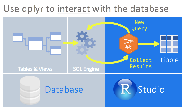
Dplyr is a fast, consistent tool for working with dataframe like objects, both in memory and out of memory. When working with big data, loading it into R might be impossible, or can substantially slow down the analysis. Instead, dplyr gives an option of handling all the data manipulations remotely, and then pulling only the resulting subset. The subset we’re interested in. Moreover, dplyr allows to interact with databases without using SQL, acting as a translator.

To use databases with dplyr, we need to install dbplyr. It’s is a relatively recent backend package which now contains all the dplyr code related to connecting to databases. More on dbplyr here and here)

install.packages("dbplyr")
install.packages("RMySQL") #for working with MySQL database

We’ll also need DBI package. It comes with dplyr automatically and provides a common interface that allows dplyr to work with many different databases using the same code. Finally, we have to install a specific backend for the database that we want to connect to.

Most commonly used backends are:

• RMySQL connects to MySQL and MariaDB

• RPostgreSQL connects to Postgres and Redshift.

• RSQLite embeds a SQLite database.

• odbc connects to many commercial databases via the open database connectivity protocol.

• bigrquery connects to Google’s BigQuery.

Establishing a connection

First, we load dplyr and one of the backend packages we’ve chosen:

library(dplyr)
library(RMySQL)

Next, we should establish the connection with DBI::dbConnect(). The arguments to DBI::dbConnect() vary from database to database, but the first argument is always the database backend.

con <- DBI::dbConnect(RMySQL::MySQL(), path = ":memory:")

It’s RSQLite::SQLite() for RSQLite, RMySQL::MySQL() for RMySQL, RPostgreSQL::PostgreSQL() for RPostgreSQL, odbc::odbc() for odbc, and bigrquery::bigquery() for BigQuery. SQLite only needs one other argument: the path to the database. Here we use the special string, ":memory:", which causes SQLite to make a temporary in-memory database.

Most existing databases live on another server. In real life the connection code will look more like this:

con <- DBI::dbConnect(RMySQL::MySQL(),
  host = "database.rstudio.com",
  user = "hadley",
  password = rstudioapi::askForPassword("Database password")
)

Old style functions are src_mysql(), src_postgres(), and src_sqlite() functions, and they still live in dplyr:

ConDplyr = src_mysql(dbname = "abc_api_efg_db", user = "annaBel", password ="mypass", host="sql.abc.com")

More on dbplyr here.

Intorduction to dplyr package

Let’s see dplyr at work using nycflights13 dataset. Load the package, and see what’s in the table “flights”.

library(nycflights13)
dim(flights) #size of a specific table
head(flights, n=2) #head of a specific tables
str(flights) #structure of a specific table

Single table verbs

Single table verbs are the commands for data manipulations within a single table of a dataset. Let’s check some important functions.

Filtering certain rows of a dataframe can be done with the help of filter() and slice() functions. filter() helps to filter rows with certain characteristics (first month, first day, departure delay is 2). Whereas slice() function picks rows by their position in a dataframe (pick rows from 1 to 5 in the example).

filter(flights, month==1, day==1, dep_delay==2)  #select a subset of rows
slice(flights, 1:5)  #select rows by position

arrange() function helps to sort information in a dataframe by fields. The first argument is always a dataframe name, then all the fields we want a DF to be arranged by. The second example arranges by arrival delay (in descending order).

arrange(dataframe name, field 1, field 2, ...)  #orders a dataframe by fields
arrange(flights, year, month, day)
arrange(flights, desc(arr_delay)) #arrange by arriving delay in descending order

In terms of working with columns, Dplyr allows to pick columns, rename them, or modify the dataframe by creating/adding new columns.

select allows rapidly subset the columns we’re interested in. This function can be used in a combination with a number of helper functions: starts_with(), ends_with(), matches(), contains().

select(dataframe name, col name 1, col name 2, ...)  #orders a dataframe by fields
select(flights, year: day) #select columns between year and day
select(flights, -(year:day)) #select except columns between year and day

One can also use select() to rename columns select(flights, tail_num= tailnumber). But it’s more common to use rename() function:

rename(flights, tail_num=tailnumber) #renames columns without dropping

We can also modify our dataframe by adding new columns that are functions of the existing columns with the help of mutate() and transmutate() functions. The latter one is used if we only want to keep new variables.

mutate(flights, gain=arr_delay-dep_delay, speed=distance/air_time*60) #renames columns without dropping

Other two handy functions to work with a single table are dictinct() and summarize():

distinct(flights, tailnum) #finds unique values in a table
distinct(flights, origin, dest)
n(x)          #the number of observations in each group
n_distinct(x) #the number of unique values in x (first(x), last(x) and nth(x,n))

Summarize() is used with affregate functions (i.e. min, max, mean,…). Dplyr also provides some special functions:

summarize(flights, delay = mean(dep_delay, na.rm = TRUE)) #collapses the data into a single variable

OBSERVATIONS: Syntaxis of all the verbs is always the same:

• the first argument is always a dataframe name
• next you describe what you do with a dataframe
• the result is a new dataframe

Grouped operations

Function group_by() breaks down a dataset into specific groups of rows. Next, when we apply the verbs above on the resulting object, they’ll be automatically applied “by group”.

For example, the following code first creates grouping by destination. Then calculates the numbers of planes and flights for each group.

destinations<- group_by(flights, dest)
summarize(destinations,
          planes = n_distinct(tailnum),
          flights = n ()
          )

Chaining

A chaining operator %>% takes the output from one function and feeds it to the first argument of the next function (turns x%>%f(y) into f(x,y). It might seem confusing at the first glance, but gets more clear when looking at an example:

Wrapping functions	Chaining equivalent
filter( summarize( select( group_by(flights, year, month, day), arr_delay, dep_delay), arr=mean(arr_delay, na.rm=TRUE), dep=mean(dep_delay, na.rm=TRUE) ), arr>30 | dep>30 )	flights %>% group_by(year,month,day)%>% select(arr_delay,dep_delay)%>% summarize( arr=mean(arr_delay, na.rm = TRUE), dep=mean(dep_delay, na.rm = TRUE) )%>% filter(arr>30|dep>30)

Two-table verbs

In practice, we usually work with many tables that contribute to the analysis, and we need tools to use them all together. In dplyr there’re two families of verbs that work with two tables at a time:

• Mutating joins (to add new fariables to one table from matching rows in another)

• Filtering joins (filter observations from one table based on whether or not they match an observation in another table)

• Set operations (combine the observations in the datasets, as if they were set elements)

Mutating joins

Allow to combine variables from multiple tables.

For example, nyflights13 dataset contains one table with flight info, and another table with mapping between abbreviations and full names. We can use join to ass the carrier names to the flight data:

flights2 <- flights %>% select (year:day, hour, origin, dest, tailnum, carrier)
flights2 %>% left_join(airlines)

Arguments: besides x and y (tables), there is also by argument that controls which variables are used to match observations in the two tables.

by =	Code	Comments
by = NULL	flights2 %>% left_join(weather)	Natural join, dplyr uses varibles that appear in both tables
by = "x"	flights2 %>% left_join(planes, by = "tailnum")	Join by some common variables, specified in char vector “x”
by = c("x"="a")	flights2 %>% left_join(airports, c("dest"="foo"))	Join by a named character vector. It will match variable x in table x to variable a in table b

Types of mutating joins

There are four types of joins that behave differently when a match is not found. Suppose we have two tables in our database, df1 and df2.

x	y
1	2
2	1

Table: df1

x	a	b
1	10	a
3	10	a

Table: df2

Inner_join(x,y) only includes observations that are both in x and y. df1 %>% inner_join(df2) results in:

x	y	a	b
1	2	10	a

Table: inner_join

Left_join(x,y) only includes all observations in x, regardless of whether they match or not. This is the most commonly used join, since it ensures that no data is lost from the primary table. df1 %>% left_join(df2) produces:

x	y	a	b
1	2	10	a
2	1	NA	NA

Table: left_join

Right_join(x,y) only includes all observations of y. In a way, it’s equivalent to left_join, but the columns will be ordered differently. df1 %>% right_join(df2) returns:

x	y	a	b
1	2	10	a
3	NA	10	a

Table: right_join

Compare it to df2 %>% left_join(df1):

x	a	b	y
1	10	a	2
3	10	a	NA

Table: left_join(df2, df1)

Full_join(x,y) only includes all observations from x and y. df1 %>% full_join(df2) gives:

x	y	a	b
1	2	10	a
2	1	NA	NA
3	NA	10	a

Table: full_join

Note: if the match is not unique, each of these joins (mutating) will add all possible combinations (the cartesian product) of the matching observations.

Filtering joins

Filtering joins match observations in the same way as mutating joins, but affect the observations, not variables. There are two kinds of such joins:

• semi_join(x, y) keeps all observations in x that have a match in y
• anti_join(x, y) drops all observations in x that have a match in y

Note: If you’re worried about what observations your joins produce, start with a semi_ or anti_join, They never duplicate, only remove observations.

Set operations

Set operations expect the x and y inputs to have the same variables and treat the observations as if they were sets.

• intersect(x, y) returns only observations in both x and y
• union(x, y) returns the unique observations in x and y
• setdiff(x, y) returns observations in x, but not in y

R to SQL translation

R	SQL
inner_join()	SELECT*FROM x JOIN y ON x.a = y.a
left_join()	SELECT*FROM x LEFT JOIN y ON x.a = y.a
right_join()	SELECT*FROM x RIGHT y ON x.a = y.a
full_join()	SELECT*FROM x FULL y ON x.a = y.a
semi_join()	SELECT*FROM x WHERE EXISTS (SELECT 1 FROM y WHERE x.a = y.a
intersect(x, y)	SELECT * FROM x INTERSECT SELECT * FROM y
union(x, y)	UNION * FROM x INTERSECT SELECT * FROM y
setdiff(x, y)	SELECT * FROM x EXCEPT SELECT * FROM y

There’s a function translate_sql() in dplyr package that allows translation of an expression to SQL:

Check here

Laziness

Dplyr is trying to be as lazy as possible. And this is a good thing: it never pools the data unless we specifically ask for it. Dplyr delays an ongoing task until the last possible moment (it collects everything together and then sends it in one step).

Example:

c1 <- filter(flights_sqlite, year == 2013, month == 1, day ==1)
c2 <- select(c1, year, month, day, carrier, dep_delay, air_time, distance)
c3 <- mutate(c2, speed = distance/air_time*60)
c4<- arrange (c3, year, month, day, carrier)

This sequence of commands never touches the database. Not until we ask for the data (for example, printing c4), that dplyr generates SQL and requests the result. But even then it only pulls 10 rows.

To pull down ALL the results, use collect() function, which returns a tbl_df(). We also can check which query was generated: c4$query.

Forcing computation

• collect() executes the query and returns the result to R
• compute() executes the query and stores temo table in the database
• collapse() turns the query into a table expression